Changing Regularizers: 2D Example
In this section we show how to change the regularizer and what are the different effects of it. The arguments of deconvolution we consider here are regularizer and $\lambda$. regularizer specifies which regularizer is used. $\lambda$ specifies how strong the regularizer is weighted. The larger $\lambda$ the more you see the typical styles introduced by the regularizers.
Initializing
This example is also hosted in a notebook on GitHub.
Load the required modules for these examples:
using DeconvOptim, TestImages, Images, FFTW, Noise, ImageView

# custom image views
imshow_m(args...) = imshow(cat(args..., dims=3))
h_view(args...) = begin
    img = cat(args..., dims=2)
    img ./= maximum(img)
    colorview(Gray, img)
end
As the next step we can prepare a noisy, blurred image.
# load test images
img = convert(Array{Float32}, channelview(testimage("resolution_test_512")))

psf = generate_psf(size(img), 30)

# create a blurred, noisy version of that image
img_b = conv(img, psf, [1, 2])
img_n = poisson(img_b, 300);

h_view(img, img_b, img_n)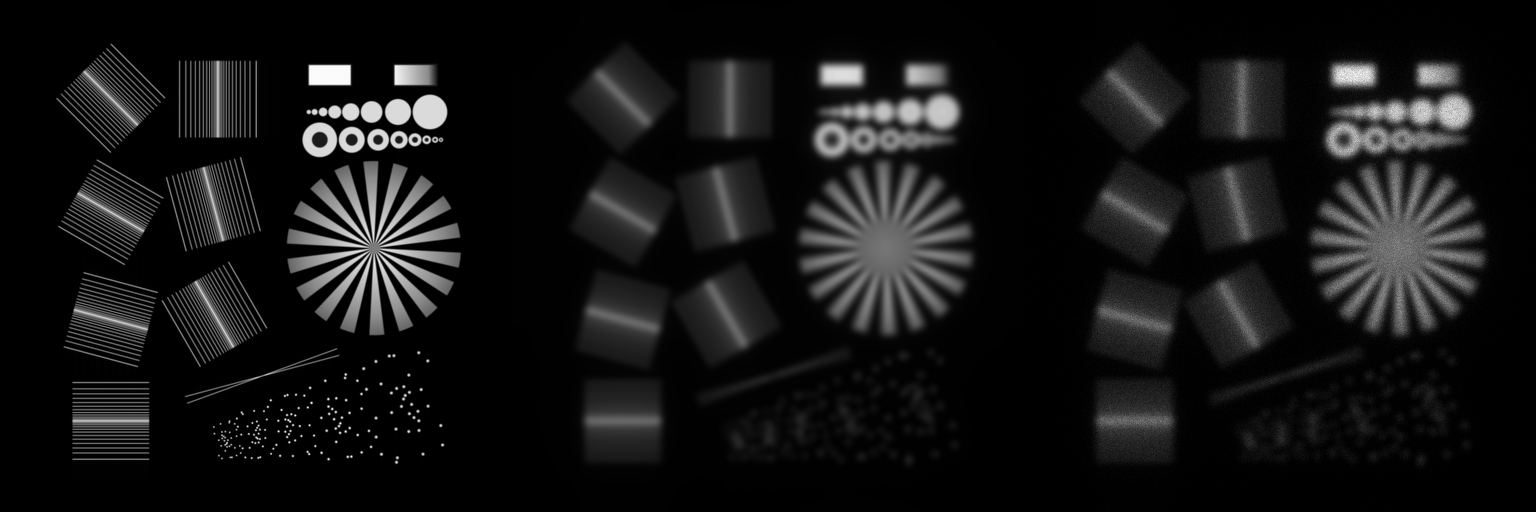
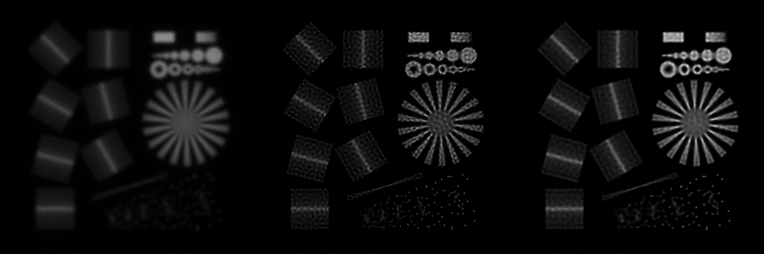
Let's test Good's roughness (GR)
In this part we can look at the results produced with a GR regularizer. After inspecting the results, it becomes clear, that the benefit of 100 iterations is not really visible. In most cases $\approx 15$ iterations produce good results. By executing GR() we in fact create a function which takes a array and returns a single value.
@time resGR100, optim_res = deconvolution(img_n, psf, regularizer=GR(), iterations=100)
@show optim_res

@time resGR15, optim_res = deconvolution(img_n, psf, regularizer=GR(), iterations=15)
@show optim_res

@time resGR15_2, optim_res = deconvolution(img_n, psf, λ=0.05, regularizer=GR(), iterations=15)
@show optim_res

h_view(img_n, resGR100, resGR15, resGR15_2)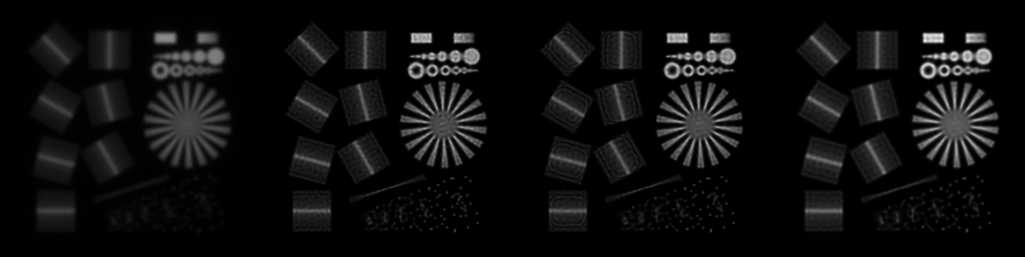
Let's test Total Variation (TV)
TV produces characteristic staircase artifacts. However, the results it produces are usually noise free and clear.
@time resTV50, optim_res = deconvolution(img_n, psf, regularizer=TV(), iterations=50)
@show optim_res

@time resTV15, optim_res = deconvolution(img_n, psf, regularizer=TV(), iterations=15)
@show optim_res

@time resTV15_2, optim_res = deconvolution(img_n, psf, λ=0.005, regularizer=TV(), iterations=15)
@show optim_res

h_view(img_n, resTV50, resTV15, resTV15_2)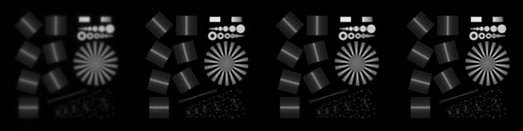
Let's test Tikhonov
Tikhonov is not defined as precisely as the other two regularizers. Therefore we offer three different modes which differ quite a lot from each other. However, the results look all very similar
@time resTik1, optim_res = deconvolution(img_n, psf, λ=0.001, regularizer=Tikhonov(), iterations=15)
@show optim_res


@time resTik2, optim_res = deconvolution(img_n, psf, λ=0.0001,
                    regularizer=Tikhonov(mode="spatial_grad_square"), iterations=15)
@show optim_res

@time resTik3, optim_res = deconvolution(img_n, psf, λ=0.0001,
    regularizer=Tikhonov(mode="identity"), iterations=15)
@show optim_res

h_view(img_n, resTik1, resTik2, resTik3)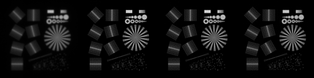
Let's test without regularizers
Usually optimizing without a regularizer is does not produce good results. The reason is, that the deconvolution tries to enhance high frequencies more and more with increasing iteration number. However, high frequencies have low contrast and therefore the algorithm mostly enhances noise content (which is present in all frequency regions).
@jldoctest
@time res100, optim_res = deconvolution(img_n, psf, regularizer=nothing, iterations=50)
@show optim_res

@time res15, optim_res = deconvolution(img_n, psf, regularizer=nothing, iterations=15)
@show optim_res

h_view(img_n, 0.7 .* res100, res15)